1. 1 简介
针对一个富斯FS-i6发射机及其接收机来学习接收机方面的知识
1.1. 1.1 发射机
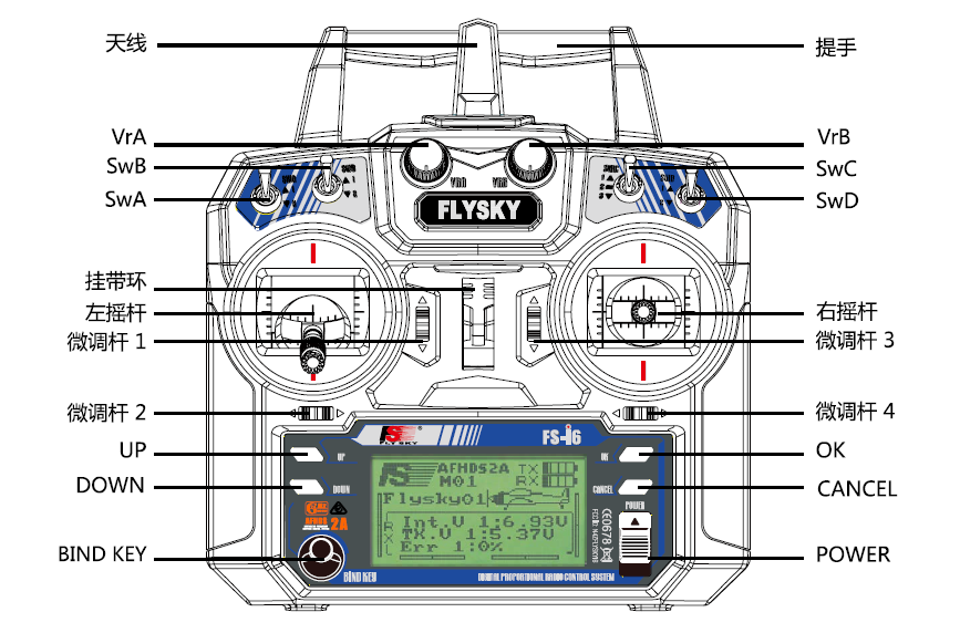
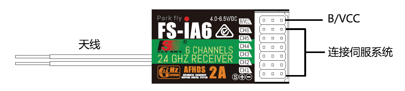
1.2. 1.2 接收机
- 型号:FS-iA6B
- 调制方式:GFSK
- 数据分辨率:1024级
- 电源标准:4.0-6.5V DC
1.3. 1.3 基本操作
- 开机:
- 先开发射机Tx
- 再开接收机Rx
- 正常情况下接收机红色指示灯常亮
针对一个富斯FS-i6发射机及其接收机来学习接收机方面的知识
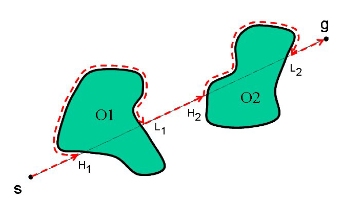
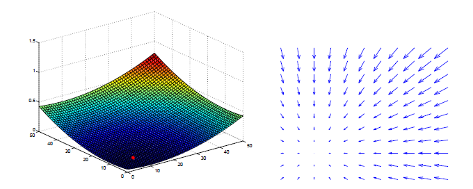
| Attractive Potential | Repulsive Potential |
|---|---|
 |
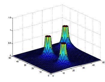 |
Combine Attractive Potential and Repulsive Potential
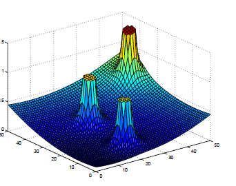
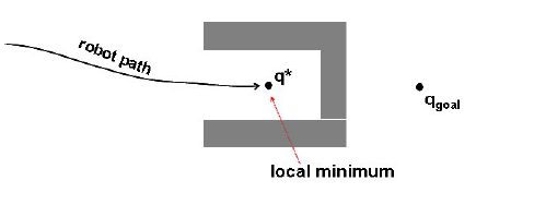
Good for static and completely known environment
Bad: may lead to a local minimum point
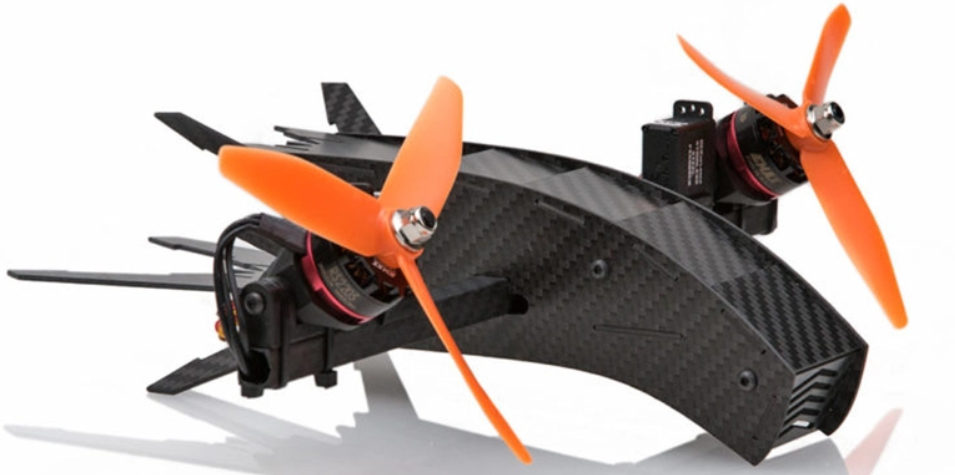
Build a bicopter(a kind of frame) like this
Principal component analysis (PCA) is a common tool for data analysis
Many problem in real world can be expressed by a small number of variables. But we don’t know that, we just collect so many data and have no ideal how to deal with hundreds of variables. Also, there will be noise in our data, which makes the problem even more complicated.
PCA is to solve this problem by identify the most meaningful basis to re-express the data. Then we can delete the less important basis( variable)
Assumption 1: bigger variance, more information
Assumption 2: If the covariance of 2 variable is big, one of them should be deleted.
Assumption 3: the principal components are orthogonal
A deque, also known as a double-ended queue, is an ordered collection of items similar to the queue. It has two ends, a front and a rear, and the items remain positioned in the collection. In a sense, this hybrid linear structure provides all the capabilities of stacks and queues in a single data structure.
Simply speaking, deques is stacks + queues
| Deque Operation | Deque Contents | Return Value |
|---|---|---|
d.is_empty() |
[] |
True |
d.add_rear(4) |
[4] |
|
d.add_rear('dog') |
['dog', 4] |
|
d.add_front('cat') |
['dog', 4, 'cat'] |
|
d.add_front(True) |
['dog', 4,'cat', True] |
|
d.size() |
['dog', 4, 'cat', True] |
4 |
d.is_empty() |
['dog', 4, 'cat', True] |
False |
d.add_rear(8.4) |
[8.4, 'dog', 4, 'cat',True] |
|
d.remove_rear() |
['dog', 4, 'cat', True] |
8.4 |
d.remove_front() |
['dog', 4, 'cat'] |
True |
In practice, we just import deque from collections module
Adding and removing from the rear is $O(1)$
Adding and removing from the front is $O(n)$
Goal: design evacuation plans at the Louvre in Paris
Difficuties: Diversity of visitors
Basic information:
What to do:
大多数生产过程的效益取决于控制的好坏,因此控制很重要。
大多数过程可以分解为一些基本环节,掌握这些环节之后我们就可以进行改造、控制,并预估性能。
总目标:对于任意外部干扰$DV$,通过调节操作变量$MV$,使被控变量$CV/PV$维持在设定值$SP$
不同的过程动态特性不相同。
自衡过程–纯滞后、单容、多容
非自衡–积分、指数
常用方程
There are two types of error:
How well dose sample error estimate true error?
We can check
e.g. with approximately $95%$ probability, true error lie in
$$
\operatorname { error } { S } ( h ) \pm 1.96\sqrt \frac { \text { errors } ( h ) \left( 1 - e r r o r { S } ( h ) \right) } { n }
$$