1. 1 Introduction
trajectory refers to a time history of position, velocity, and acceleration for each degree of freedom.
Concern:
- Easy description:just desired goal position and orientation
- How to generating and representing in computer
2. 2 General consideration
- Huamn-interface. Consider tool frame ${T}$ , in which a user would think and design path.
- Path include many intermediate points (position and orientation)
- Want a smooth path, first derivative even second derivative. jerky motions tend to cause increased wear on the mechanism andcause vibrations by exciting resonances in the manipulator
3. 3 Joint-Space Schemes
First get the via points and then convert it to a set of joint angle by inverse kinematics
Joint space schemes is the easiest to compute.
3.1. 3.1 Cubic Polynomials
Some constrains:
- $θ(0) = θ_0$ initial
- $θ(t_f ) = θ_f$ final
- $\dotθ(0) = 0$ continuous in velocity
- $\dotθ(t_f ) = 0$ continuous in velocity
apply
$$
θ(t) = a_0 + a_1t + a_2t^2 + a_3t^3solve the problem
$$
to solve the problem (between two points)
3.2. 3.2 Cubic polynomials for a path with via points
What if we wish to specfify the intermediate via points? (between many points)
constrains becoms
- $θ(0) = θ_0$ initial
- $θ(t_f ) = θ_f$ final
- $\dotθ(0) = \dot\theta_0$ continuous in velocity
- $\dotθ(t_f ) = \dot\theta_f$ continuous in velocity
But how we choose the intermediate velocity? There are some method:
Specified by user
Choose by computer
If the slope of lines change sign at via point $\to$zero velocity
if the slope of lines does not change sign$\to$average velocity
3.3. 3.3 Linear function with parabolic blends
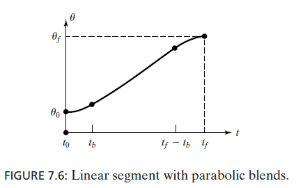
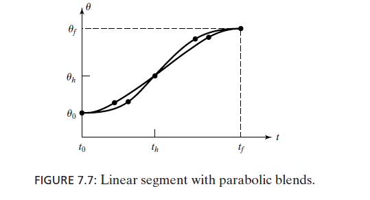
$$
\ddotθ\times t_b =\frac{θ_h − θ_b}{t_h − t_b}
$$
$$
θ_b = θ_0 + \frac12\ddotθ\times t_b^2
$$
There are 2 equations and 6 variabels
So, given $\theta_f ,\theta_0, t_h$, choose $\ddot\theta\to$we can calculate $t_b$
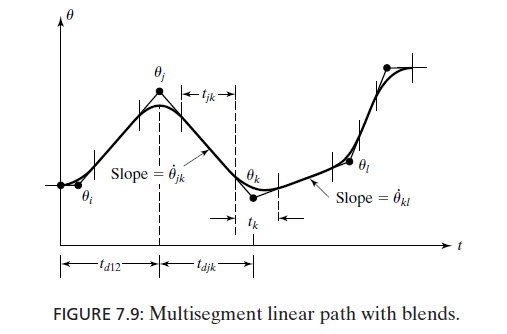
3.4. 3.4 Linear function with parabolic blends for a path with via points
Consider there an arbitrary number of via points
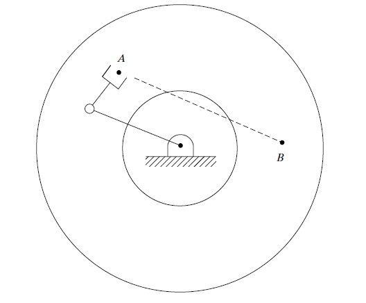
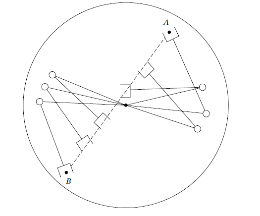
4. 4 Cartesian-Space Schemes
In Joint-Space, the spatial shape of path taken by the end-effector will be complicated
In Cartesian-Space, we can also specify shape of the path. Line\Circular\Sinusoidal
However, Cartesian schemes are more computationally expensive because inverse kinematics must be solved at real time
5. 5 Geometric Problems with Cartesian Paths
- Intermediate points unreachable
- High joint rates near singularity
- Start and goal reachable in different solutions