1. 1 Introduction
Premise: Know the means to calculate joint-position correspond to desired end-effector motions.
Problem: How to cause the manipulator acually to perform these desired motions.
Solution 1: Linear control system.
- In fact, non-linear is more usual, linear control is just a approximate methods
- It’s resonable to make such approximation, so lineat control methods are the ones most often used in industrial practice.
- Learn linear first is good for later study
2. 2 Control-Law Partitioning
Partitioning Method (2 parts):
- model-based portion: make use of supposed knowledge of m,b,k, to make the system appear as a unit mass$\to$ servo portion simple.
- servo portion: make use of feedback to modify the behavior of the system
A open-loop equation of motion for the system:
$$
m \ddot { x } + b \dot { x } + k x = f
$$
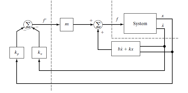
The model-based portion of the control:
$$
f = \alpha f ^ { \prime } + \beta
$$
and we choose(because we want to make the )
$$
\begin{array} { l } { \alpha = m } \ { \beta = b \dot { x } + k x } \end{array}
$$
finally we get $\ddot { x } = f ^ { \prime }$
Graphiclly,we transform a system like this
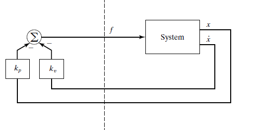
into a system easier
What we need to do is design a control law to compute $f ^ { \prime } = - k _ { v } \dot { x } - k _ { p } x$
so it yields
$$
\ddot { x } + k _ { v } \dot { x } + k _ { p } x = 0
$$
2.1. Conclusion
- get the system‘s parameters
- find $\alpha ,\beta$
- calculate $k_v,k_p$ depend on the requirement
2.2. 3. Trajectory-Following Control
Know: trajectory, a funciton of time $x_d(t)$ and we can get $\dot x_d, \ddot x_d $as well
Define: $e=x_d-x$
Design $f ^ { \prime } = \ddot { x } _ { d } + k _ { v } \dot { e } + k _ { p } e$
Get: $\ddot { x } = \ddot { x } _ { d } + k _ { v } \dot { e } + k _ { p } e$
So, we can choose coefficients and design any response we want