1. 1 Introduction
End-effector moves with a spatial velocity, and it’s a consequnece of all individual joint velocities.
Here, we introduce the relationship between joint velocities and end-effector‘s velocity
In kinematics, we care about the pose, now we care about velocity
2. 2 Manipulator Jacobian
2.1. 2.1 Overview
Jocabian:
$$
J = \frac { \partial f } { \partial x } = \left( \begin{array} { c c c } { \frac { \partial y _ { 1 } } { \partial x _ { 1 } } } & { \cdots } & { \frac { \partial y _ { 1 } } { \partial x _ { n } } } \ { \vdots } & { \ddots } & { \vdots } \ { \frac { \partial y _ { m } } { \partial x _ { 1 } } } & { \cdots } & { \frac { \partial y _ { m } } { \partial x _ { n } } } \end{array} \right)
$$
In manipulator, $f$ (end-effector pose) and $x$ (joint variables) are all vector:
$$
\frac { \mathrm { d } p } { \mathrm { d } q } = \mathrm { J } ( q ) \to \mathrm { d } \boldsymbol { p } = \boldsymbol { J } ( \boldsymbol { q } ) \mathrm { d } \boldsymbol { q }
$$
and divide through by $dt$
$$
\begin{aligned} \frac { \mathrm { d } p } { \mathrm { d } t } & = J ( q ) \frac { \mathrm { d } q } { \mathrm { d } t } \to \dot { p } = J ( q ) \dot { q } \end{aligned}
$$
Jocabian is a $J \in R^{6\times N} $ ($6$ for enviroment, $N$ for n joints) matrix
2.2. 2.2 Under- and Over-Actuated Manipulators
- Under-Actuated: accepting that some Cartesian degrees of freedom are not controllable
- Over-Actuated: multiple solution, so find a least-squares solution
3. 3 Jocabian: Numerical Properties
$$
\dot{p}=J ( q ) \dot { q }\
\dot { q } = J ( q ) ^ { - 1 } \nu
$$
3.1. 3.1 Singularities
Singularities occur when the robot is at maximum reach or when one or more axes become
aligned resulting in the loss of degrees of freedom. aka $det(J(q))=0$
If robot is close to a singularity, some end-effector velocities require very high joint rates
3.2. 3.2 Manipulability
4. 4 Inverse Jocabian: generate paths
4.1. 4.1 Resolved-Rate Motion Control
Resolved-rate motion control is a simple and elegant algorithm to generate straight
line motion
It make use of $\dot { \boldsymbol { q } } = J ( \boldsymbol { q } ) ^ { - 1 } \boldsymbol { \nu }$ to map resovle desired Cartesian velocity to joint velocity
Control scheme:
- first $\dot { \boldsymbol { q } } ^ { * } \langle k \rangle = J ( \boldsymbol { q } \langle k \rangle ) ^ { - 1 } \nu ^ { * }$ computes the required joint velocity as a function of the manipulator and disired end-effector velocity $\nu ^ { * }$
- then $q ^ { * } \langle k + 1 \rangle \leftarrow \boldsymbol { q } \langle k \rangle + \delta _ { t } \dot { \boldsymbol { q } } ^ { * } \langle k \rangle$ perform intergration to give desired joint angle for next step.
5. 5 Jocabian: Transform Force from End to Joint
6. 6 Jocabian: Inverse Kinematics
If a robot don’t meet some specification:
- have 6 joints
- have a spherical wrist
Then, it’s hard to give a explicit solution. So we introduce general numerical solution based on:
- forward kinematics
- the Jacobian transpose
Idea: compute by error
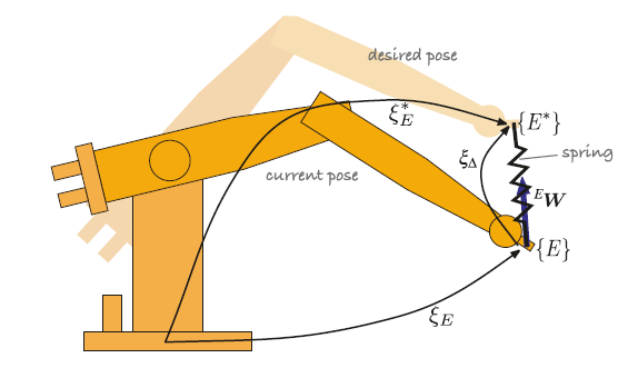
Notation: actual pose $\xi _ { E } = \mathcal { X } ( q )$ , desired pose $\xi _ { E } ^ { * }$ , error between them:$\xi _ { \Delta }$ (also can be described by a spatial displacement)
$$
^ { E } \Delta = \Delta \left( \xi _ { E } , \xi _ { E } ^ { * } \right) = ( t , \hat { v } \theta ) \in \mathbb { R } ^ { 6 }
$$
How to compute?
imagine a spring between two pose, which is pulling and twisting (wrench) the end-effector proportional to the spatial displacement $\to ^ { E } \boldsymbol { W } = \gamma ^ { E } \boldsymbol { \Delta }$
the wrench is resolved to generalized joint forces $\to\boldsymbol { Q } = _{}^{E}\textrm{} \boldsymbol { J } ( \boldsymbol { q } ) ^ { T } \boldsymbol { W }$
assume joint velocity just be proportional to the forces $\to \dot { q } = Q / B (a \ coefficient)$
wrap up: $\dot { \boldsymbol { q } } = \frac { 1 } { B } \boldsymbol { J } ( \boldsymbol { q } ) ^ { T } \Delta \left( \mathcal { K } ( \boldsymbol { q } ) , \xi _ { E } ^ { * } \right)$
we can solve it interatively by:
$$
\begin{aligned} \delta _ { q } \langle k \rangle = \alpha J ( \boldsymbol { q } \langle k \rangle ) ^ { T } \Delta \left( \mathcal { K } ( \boldsymbol { q } \langle k \rangle ) , \xi _ { E } ^ { * } \right )\
\boldsymbol { q } \langle k + 1 \rangle \leftarrow \boldsymbol { q } \langle k \rangle + \delta _ { q } \langle k \rangle \end{aligned}
$$until the norm of the update $\left| \delta _ { q } \langle k \rangle \right|$ is sufficiently
pratically above algorithm is slow and sensitive to $\alpha$ ,so we imporve it by:
formulate this as a least-squares problem: $\to E = \boldsymbol { \Delta } ^ { T } M \Delta$
we want to minimize the scalar cost
where $M = \operatorname { diag } ( m ) \in \mathbb { R } ^ { 6 \times 6 }$ and $m$ is the mask vector
update becomes :$\delta _ { q } \langle k \rangle = \left( J ( \boldsymbol { q } \langle k \rangle ) ^ { T } \boldsymbol { M } \boldsymbol { J } ( \boldsymbol { q } \langle k \rangle ) \right) ^ { - 1 } \boldsymbol { J } ( \boldsymbol { q } \langle k ) ) ^ { T } \boldsymbol { M } \Delta \left( \mathcal { X } ( \boldsymbol { q } \langle k \rangle ) , \xi _ { E } ^ { * } \right)$
impove above performance near singularities by introducing a damping constant λ:
$$
\delta _ { q } \langle k \rangle = \left( J ( \boldsymbol { q } \langle k \rangle ) ^ { T } \boldsymbol { M } \boldsymbol { J } ( \boldsymbol { q } \langle k \rangle ) +\lambda I_{N\times N}\right) ^ { - 1 } \boldsymbol { J } ( \boldsymbol { q } \langle k ) ) ^ { T } \boldsymbol { M } \Delta \left( \mathcal { X } ( \boldsymbol { q } \langle k \rangle ) , \xi _ { E } ^ { * } \right)
$$
An effective way to choose $\lambda$ is to test whether or not an iteration reduces the error