We need $x$ but we do have is only $y$. What can we do?
- Design $u$ as if we had $x$
- Figure out $x$ from $y$
1. Assume We Got $x$
We can design the $k_1$ and $k_2$ to make the eigenvalue of the closed-loop system to be desired (negative)
e.g. If we want to the eigen value of the $-1$, then, $\varphi(\lambda)=(\lambda+1)(\lambda+1)=\lambda^{2}+2 \lambda+1$
and we got $\chi_{A-B K}=\lambda^{2}+k_{2} \lambda+k_{1}$
so just let $k_2=2$ and $k_1=1$, the system would be stable
To say it in another way, we place the pole of the system on the desired position
Still, we have some question about the method?
- This method is not always possible
- The system needs to be controllable
- It’s a science and art of picking the eigenvalue
- No clear-cut answer
2. Controllability
The key matter here is the $B$ matrix, how rich is $B$ that we can control the system.
If we write the system this way
$$
\begin{aligned}
\begin{array}{l}
x_{1}=A x_{0}+B u_{0}=B u_{0}\
x_{2}=A x_{1}+B u_{1}=A B u_{0}+B u_{1} \
x_{3}=A x_{2}+B u_{2}=A^{2} B u_{0}+A B u_{1}+B u_{2}
\end{array}
\end{aligned}
$$
Then we can transform the system into
$$
x=\Gamma u=[B \ AB \ …\ A^{n-1}B]u
$$
if $Rank(\Gamma)=n$, it’s possible to fully control the system
if the system can be fully controlled, then we can put arbitrary pole
$$
Rank(\Gamma)\to Fully \ Control \to Arbitrary\ Pole
$$
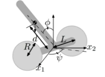
Application: Segway Robots
Segway robots is simply unicycle+Inverted Pendulum+…
Model the system
$$
\begin{array}{l}
x=\left[\begin{array}{lllllll}
x_{1} & x_{2} & v & \psi & \dot{\psi} & \phi & \dot{\phi}
\end{array}\right]^{T} \
u=\left[\begin{array}{ll}
\tau_{L} & \tau_{R}
\end{array}\right]^{T}
\end{array}
$$
After linearization, $Rank(\Gamma)=6<7$, so the system is not fully controllalityThat’s because unicycle mess up while linearization around (0,0)
So we can shave off the $x_1$ and $x_2$. Now the system is fully controlled
- In this way, we only control the curvature of the path
3. Observability
Actually, we don’t the real value of $x$, so we need sensor or observer to estimate $x$
Luenberger observer: predictor + corrector
$$
\dot{ \hat{x}}=A\hat x+L(y-C \hat x)
$$
predictor + corrector
Does it work?
How to pick $L$
We want to stabilize the estimation error, $e=x-\hat x$
$$
\dot e=(A-LC)e
$$
so the it should be $Re(eig(A-LC))<0$
The system is completely observable if it is possible to recover the initial state from the output
$$
\Omega=\left[\begin{array}{c}
C \
C A \
\vdots \
C A^{n-1}
\end{array}\right]
$$
$$
rank(\Omega)=n
$$
4. Put it Together!
Now we have good building blocks
- controllability, observability, state feedback, observers, pole-placement
How do we put everything together?
Answer: Separation Principle
First of all, we need to make sure that our linear system is CC and CO
Design state feedback controller as if we had $x$
let $u=-Kx$, and design $\dot x=(A-BK)x$
- Estimate $x$ using observer, make sure the error estimation is zero
$\dot e=(A-LC)e$
- Analyze their joint dynamics, notice that $e=x-\hat x$
Then $\dot{x}=A x-B K \hat{x}=A x-B K(x-e)=(A-B K) x+B K e$
now we want $x$ and $e$ both go to zero
$$
\left[\begin{array}{c}
\dot{x} \
\dot{e}
\end{array}\right]=\left[\begin{array}{cc}
A-B K & B K \
0 & A-L C
\end{array}\right]\left[\begin{array}{c}
x \
e
\end{array}\right]
$$
Since this is an upper triangular block-matrix. So the eigenvalues are given by the diagonal blocks
EVERYTHING WORKS because they are separated
5. Practical Considerations
- Eigenvalue Selection
- Observer should be faster than the controller.
- So we need to make sure the eigenvalue of observer smaller than the controller
- Reference Tracking
- We want to move the robots to $\theta_d$, so the $e$ became $\begin{array}{c} \theta-\theta{_d} \\dot \theta \end{array}$
- transform the system into regular system, and apply regular methodology
Beyond Pole Placement
The methodology we developed does not need to be based on pole placement
e.g. $K$ could be calculated by using LQ optimal control
$L$ could be calculated by using the Kalman Filter
6. Example
6.1. Part 1: Design
We have a system $\dot x=Ax$, and $eig(A)=0$, so the system is unstable.
Hence we introduce control.
- See what we can control, and write down the $B$ matrix to check is this system controllable by checking the $\Gamma$ Matrix
- If the system is uncontrollable, then we should introduce more motors
- Design state feedback control $u=-Kx$, we get $\dot x=(A-BK)x$
- Pick favorite eigen value, calculate $K$
- Choose what we can “see”, what we can sensor, measure. In this we get our $C$ matrix to check is this system observable by checking the $\Omega$ matrix
- Design the estimator $\dot {\hat {x}}=A \hat{x}+B u+L(y-C \hat{x})$
we get $\dot e=(A-LC)e $ and calculate $L$
6.2. Part 2: Executing
Loop
- Initialize $t=t_0 ,x=x_o,\hat x=\hat{x_0}$
- Start Loop (dt increments)
- read the output
- Compute control signal $u=-K\hat x$
- send the control signal to the motors
- output and compute control signal $u=-K\hat x$
- update the $\hat x$ using $\dot {\hat {x}}=A \hat{x}+B u+L(y-C \hat{x})$ and $\hat{x}{k+1}=\hat{x}{k}+d t \hat{x}$