Data-Regression

1. 1 Introduction

In statistical modeling, regression analysis is a set of statistical processes for estimating the relationships among variables.

$$
\left{\begin{array}{l}{y=\beta_{0}+\beta_{1} x+\varepsilon} \ {E \varepsilon=0, D \varepsilon=\sigma^{2}}\end{array}\right.
$$

2. 2 the Develop of Algorithm

2.1. Problem set

$$
\mathbf{X}=\left[ \begin{array}{cccc}{x_{11}} & {x_{12}} & { . .} & {x_{1 m}} \ {x_{21}} & {x_{22}} & {\dots} & {x_{2 m}} \ {\ldots} & {\cdots} & {\cdots} & {\cdots} \ {x_{n 1}} & {x_{n 2}} & {\dots} & {x_{n m}}\end{array}\right]
$$

$$
Y=\left(y_{1} \quad y_{2}\right)=\left[ \begin{array}{cc}{y_{11}} & {y_{12}} \ {y_{12}} & {y_{22}} \ {\cdots} & {\cdots} \ {y_{1 n}} & {y_{2 n}}\end{array}\right]
$$

$$
B=\left(b_{1} \quad b_{2}\right)=\left[ \begin{array}{cc}{b_{11}} & {b_{21}} \ {b_{12}} & {b_{22}} \ {\dots} & {\dots} \ {b_{1 m}} & {b_{2 m}}\end{array}\right]
$$

$$
E=\left(e_{1} \quad e_{2}\right)=\left[ \begin{array}{cc}{e_{11}} & {e_{21}} \ {e_{12}} & {e_{22}} \ {\cdots} & {\cdots} \ {e_{1 n}} & {e_{2 n}}\end{array}\right]
$$

$$
\boldsymbol{Y}=\boldsymbol{X} \boldsymbol{B}+\boldsymbol{E} ; \quad y_{1}=\boldsymbol{X} \boldsymbol{b}{1} ; \quad y{2}=\boldsymbol{X} \boldsymbol{b}_{2}
$$

we know (2) and (3), we want to get (6) , so we need to solve (4) and (5)

2.2. 2.1 OLS

Ordinary least squares

• Constraint: $min(error)​$
  $$
  e=y-\mathbf{X} b \quad \Rightarrow \quad \min \left(e^{\prime} e\right)
  $$

• Solution: Solved by Lagrange Multiplier
  $$
  b=\left(X^{\prime} X\right)^{-1} X^{\prime}{y}
  $$

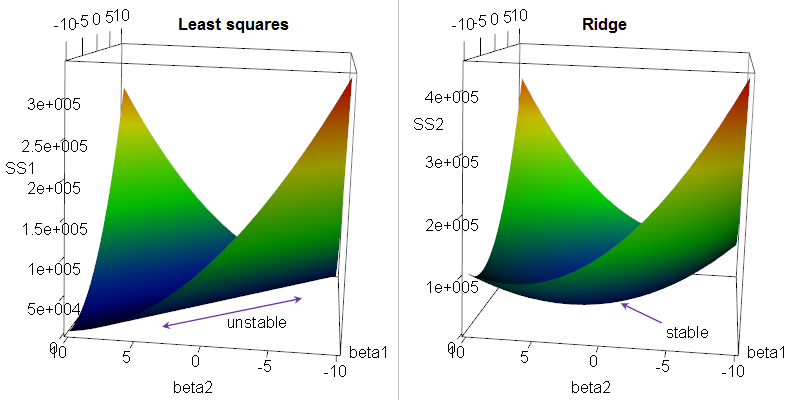
• Problem: if there are multi -collinearity in $\mathbf{X}​$ , $b​$ will be very big, like $\infin​$

2.3. 2.2 RR

Ridge Regression: solve the problem in the OLS, add some constraint for $b​$

• Constraint: $min(error \ &\ b​$)
  $$
  e=y-\mathbf{X} b \quad \Rightarrow \quad \min \left(e^{\prime} e+kb^{\prime}b \right )
  $$

• Solution:
  $$
  \hat{\boldsymbol{\beta}}(\mathrm{k})=\left(X^{\prime} X+k I\right)^{-1} X^{\prime} y
  $$

• Problem: how to choose $k$ is a problem

Why it called ridge?

2.4. 2.3 PCR

Principal Component Regression: Often the principal components with higher variances are selected as regressors

• Constraint: Apply PCA to $\mathbf{X}$, get component matrix $\mathbf{F}$
  $$
  \mathbf{F}=\mathbf{X}_{0} \mathbf{U}
  $$

• Solution:
  $$
  \hat{\gamma}=\left(\mathbf{F}^{\prime} \mathbf{F}\right)^{-1} \mathbf{F}^{\prime} \mathbf{Y}
  $$

• Problem: for the purpose of predicting the outcome, the principal components with low variances may also be important, in some cases even more important. MORE

2.5. 2.4 PLS

Partial least squares regression: it finds a linear regression model by projecting the predicted variables and the observable variables to a new space

Underlying model of PLS:

$$
\begin{aligned} X &=T P^{\mathrm{T}}+E \ Y &=U Q^{\mathrm{T}}+F \end{aligned}
$$

• Constraint:

1. Variances of $T$ and $U$ should be as big as possible
2. Correlation of $T​$ and $U​$ should be as big as possible

• Combine 1. and 2. , we want covariance of $T$ and $U​$ be as big as possible