1. 1 Introduction
Spinning Up brought by OpenAI is a good resource for learning reinforcement learning.
The goal of Spinning up is to ensure AI is safe developed and help people to learn Deep RL which has a pretty high barrier to entry
In a nutshell, RL is the study of agents and how they learn by trial and error. It formalizes the idea that rewarding or punishing an agent for its behavior makes it more likely to repeat or forego that behavior in the future.
Learning Types:
- supervised:given x and y, find $f()$
- unsupervised:given x, find $cluster$
- reinforcement:given x and z, find decision $f()$ to generate y
- difference from supervised learning: delayed reward that is your movement will affect later world. about time and sequence
Markov decision process (MDP) :
- states: things described the world
- actions: things you can do
- model: rules, physics of the world
- reward: a scaler value to value the state
- policy: what we want to learn, $\pi^{\star}(state)\to action$ ,the action can maximize the cumulative reward.
- when moving in the grid map, agent should avoid $-negative$ reward and get $+positive$ reward
- You need to set the reward carefully
- Even if you are in the same state, your action will be different for different step(time) you can take later. E.g. if you have only 3 steps to go, you may take action risky, $\pi^{\star}(state,time)\to action$
2. 2 Key Concepts
2.1. 2.1 What can RL do
- Teach computers to control robots in simulation and real world
- Create breakthrough AI for sophisticated strategy games (Go/Dota)
- …
2.2. 2.2 Terminology
Main loop of RL:
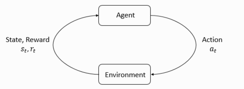
state $s$ : complete description of the state of the world
represented by a vector, matrix or tensor
Grid map e.g. $4\times3$
observation $o$ : partial description of a state
represented by a vector, matrix or tensor
Action space: The set of all valid actions
Discrete action space: Go and Atari
Continuous action space: Control a robot
Policies: rule used by an agent to decide what actions to take
deterministic $a_{t}=\mu\left(s_{t}\right)$
stochastic $a_{t} \sim \pi\left(\cdot | s_{t}\right)$ : sampling action $+$ computing $\log \pi_{\theta}(a | s)$ , which means your action may not be execute $100%$ that is uncertainty
Catergorical policies: discrete, jsut like a classifier, output are probabilities vector
diagonal Gaussian policies: continuous
The policy is trying to maximize reward
Trajectories: $\ $ $\tau$ is a sequence of states and actions in the world
$\tau=\left(s_{0}, a_{0}, s_{1}, a_{1}, \dots\right)$
Reward and Return: depends on the current state, the action just taken, and the next state of the world
$r_{t}=R\left(s_{t}, a_{t}, s_{t+1}\right)$ but ususally simplified to $r_{t}=R\left(s_{t}\right)$
goal of the agent is to maximize cumulative reward over trajectory $R(\tau)=\sum_{t=0}^{T} r_{t}$
if the time is infinite, we should add a factor to the cumulative reward or it will go $\infty$ , so we should $R(\tau)=\sum_{t=0}^{\infty} \gamma^{t} r_{t}$
The RL Problem: select a policy which maximized expected return
Value Funciton: know the value of a state
On-Policy Value Function $V^{\pi}(s)$
On-Policy Action-Value Function $Q^{\pi}(s, a)$
start with random action
Optimal Value Function $V^{*}(s) $
Optimal Action-Value Function $Q^{*}(s, a)$
Bellman Equations
basic idea: The value of your starting point is the reward you expect to get from being there, plus the value of wherever you land next.
$V^{*}(s)=\max {\pi} \underset{\tau \sim \pi}{\mathrm{E}}\left[R(\tau) | s{0}=s\right]$
$n$ equations and $n$ unknown
3. 3 Kinds of RL Algorithms
3.1. 3.1 Taxonomy

Model-Based RL:
- Upside: allows the agent to plan by thinking ahead. Example: AlphaZero
- Downside: the given model is different from the real enviroment the agent works.
Model-Free RL:
- Upside: easier to implement and tune, more popular
3.2. 3.2 What to Learn
3.2.1. 3.2.1 Model-Free RL
Policy Optimization: On policy
A2C / A3C, gradient ascent
PPO, updates indirectly
Q-Learning: Off policy
learn an approximator $Q_{\theta}(s, a)$ for the optiaml action-value function.
DQN
C51
Trade-offs:
Policy: these kind of algorithm optimize for the thing we want directly.
Q-Learning’s result is unstable, which means it may be better sometimes but maybe worse other times.
3.2.2. 3.2.2 Model-Based RL
- Pure Planning: compute a new plan each time, execute the first action and discards the rest of it.
- Expert Iteration: updated version of Pure-Planning
- Data Augmentation for Model-Free Methods
- …
4. 4 Policy Optimization
4.1. 4.1 Deriving some Math
Here we consider the case of stochastic, parameterized policy.
Aim: maximize the expected return $J\left(\pi_{\theta}\right)=\underset{\tau \sim \pi_{\theta}}{E}[R(\tau)]$
How: optimize by gradient ascent: $\theta_{k+1}=\theta_{k}+\alpha \nabla_{\theta} J\left.\left(\pi_{\theta}\right)\right|{\theta{k}}$ ,which means we need an expression for the policy.
Program:
- Making the policy network
- make core policy network
- make action selection
- Making the Loss Function
- Running one Epoch of Training