1. 1 Introduction
Testing whether a hypothesis is true or false by calculating the probability of an event in a prolonged experiment is known as frequentist statistics
- An experiment with an infinite number of trials guarantees $p$ with absolute accuracy
- It’s not practial to conduct an experiment with an infinite number of trials
- deciding the value of this sufficient number of trials is a challenge
- If we can determine the confidence of the estimated $p$ , it will allow us to decide whether to
- accept the conclusion
- extend the experiment with more trials until it achieves sufficient confidence
- prior beliefs (for example, coins are usually fair and the coin used is not made biased intentionally, therefore $p≈0.5$)
- play a significant role in shaping the outcome of a hypothesis test
- However, it ==can’t== be used along with frequentist statistics
2. 2 Bayesian Learning
Consider the flip coin experiment, if you flip the coin $10$ times, there are 2 case:
5 heads and 5 tails
more confidence about that $p=0.5$
$x$ head and $10-x$ tails
Now you have 2 options
- frequentist statistics :Neglect prior beliefs, just based on data
- Bayesian Learning :Adjust your belief according to observation
2.1. 2.1 Bayes’ Theorem
Bayes’ theorem
$$
P ( \theta | X ) = \frac { P ( X | \theta ) P ( \theta ) } { P ( X ) }
$$
- $P ( \theta )$ Prior Probability is the probability of the hypothesis $\theta$ being true
- $P ( X | \theta )$ Likelihood is the conditional probability of the evidence given a hypothesis
- $P ( X )$ Evidence :a summation (or integral) of the probabilities of all possible hypotheses
- $P ( \theta | X )$ Posteriori probability
2.2. 2.2 Application1: MAP
Used to confirm the valid hypothesis using posterior probabilities
$$
\begin{aligned} \theta { M A P } & = \operatorname { argmax } { \theta } P \left( \theta { i } | X \right) \ & = \operatorname { argmax } { \theta } \left( \frac { P ( X | \theta { i } ) P \left( \theta { i } \right) } { P ( X ) } \right) \end{aligned}
$$
$P(x)$ is independent of $\theta$ . Therefore, we can simplify the $\theta_{MAP} $ to
$$
\theta_ { M A P } = \operatorname { argmax } { \theta } \left( P ( X | \theta { i } ) P \left( \theta _ { i } \right) \right)
$$
2.3. 2.3 How to Achieve the Goal
For the $P ( X | \theta _ { i } )$ part
Use $MLE$
$$
\frac { d } { d \theta } \ln P (X | \theta ) = 0
$$
For the $P \left( \theta _ { i } \right)$ part
if the hypothesis space is continuous, it will be endless hypothesis.
So in practical, we use approximation techniques : Beta prior distribution
$$
P ( \theta ) = \frac { \theta ^ { \alpha - 1 } ( 1 - \theta ) ^ { \beta - 1 } } { B ( \alpha , \beta ) }
$$
- $B ( \alpha , \beta )$ acts as the normalizing constant
2.4. 2.4 Example
As a Binomial probability example
$$
P ( k , N | \theta ) = \left( \begin{array} { c } { N } \ { k } \end{array} \right) \theta ^ { k } ( 1 - \theta ) ^ { N - k }
$$
$$
P ( \theta ) = \frac { \theta ^ { \alpha - 1 } ( 1 - \theta ) ^ { \beta - 1 } } { B ( \alpha , \beta ) }
$$
So the posterior
$$
\begin{aligned} P ( \theta | N , k ) & = \frac { P ( N , k | \theta ) \times P ( \theta ) } { P ( N , k ) } \ & = \frac { \left( \begin{array} { c } { N } \ { k } \end{array} \right) } { B ( \alpha , \beta ) \times P ( N , k ) } \times \theta ^ { ( k + \alpha ) - 1 } ( 1 - \theta ) ^ { ( N + \beta - k ) - 1 } \end{aligned}
$$
and consider it as a new Beta prior distribution
$$
P ( \theta | N , k ) = \frac { \theta ^ { \alpha { n e w } - 1 } ( 1 - \theta ) ^ { \beta { n e w } - 1 } } { B \left( \alpha { n e w } , \beta { n e w } \right) }
$$
3. 3 Bayes Optimal Classifier
Given new instance $x$, the hypothesis we get previously $h _ { M A P } ( x )$ may be not the most probable classification.
e.g.1
$$
P \left( h { 1 } | D \right) = 0.4 , P \left( h { 2 } | D >\right) = 0.3 , P \left( h _ { 3 } | D \right) = 0.3
$$
New instance$$
h { 1 } ( x ) = + , h { 2 } ( x ) = - , h _ { 3 } ( x ) = -
$$
Bayes optimal classifier tell us that we should find:
$$
\arg \max { v { j } \in V } \sum { h { i } \in H } P \left( v { j } | h { i } \right) P \left( h _ { i } | D \right)
$$
e.g.1
$$
P \left( h { 1 } | D \right) = 0.4 , P ( - | h { 1 } ) = 0 , >P ( + | h { 1 } ) = 1 \ P \left( h { 2 } | D \right) = 0.3 , >P ( - | h { 2 } ) = 1 , P ( + | h { 2 } ) = 0 \ P \left( h { >3 } | D \right) = 0.3 , P ( - | h { 3 } ) = 1 , P ( + | h { 3 >} ) = 0
$$
therefore
$$
\begin{aligned} \sum { h { i } \in H } P ( + | h { i } ) P >\left( h { i } | D \right) & = .4 \ \sum { h { i } \in H } P >( - | h { i } ) P \left( h _ { i } | D \right) & = .6 >\end{aligned}
$$
so we choose $-$ as the classification
4. 4 Navie Bayes Classifier
When to use:
- Large training set available
- Attributes are independent
- Used in diagnosis and text classification
Navie Bayes assumption:
$$
P \left( a { 1 } , a { 2 } \ldots a { n } | v { j } \right) = \prod { i } P \left( a { i } | v { j } \right)
$$
Bayes MAP
$$
\begin{aligned} v { M A P } & = \underset { v { j } \in V } { \operatorname { argmax } } \frac { P \left( a { 1 } , a { 2 } \ldots a { n } | v { j } \right) P \left( v { j } \right) } { P \left( a { 1 } , a { 2 } \ldots a { n } \right) } \ & = \underset { v { j } \in V } { \operatorname { argmax } } P \left( a { 1 } , a { 2 } \ldots a { n } | v { j } \right) P \left( v { j } \right) \end{aligned}
$$
Navie Bayes Classifier
$$
v { N B } = \underset { v { j } \in V } { \operatorname { argmax } } P \left( v { j } \right) \prod { i } P \left( a { i } | v _ { j } \right)
$$
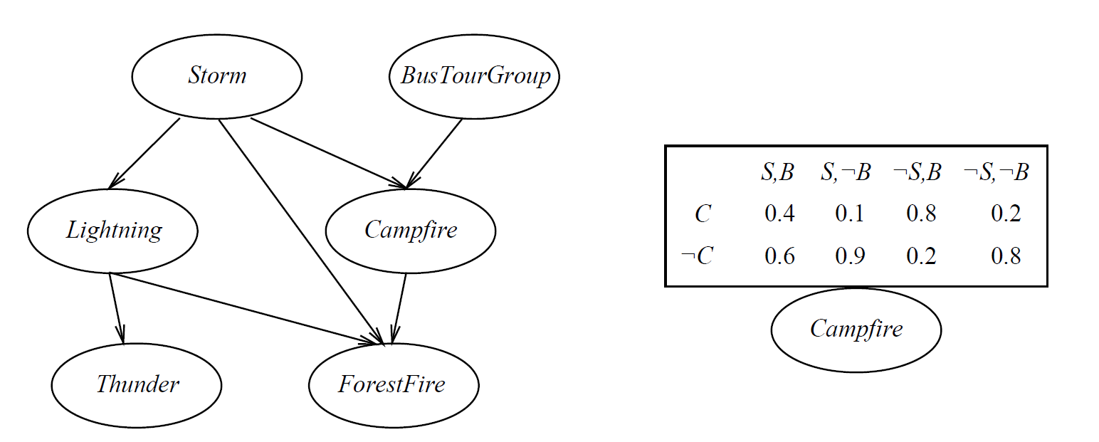
5. 5 Bayesian Belief Networks
Improve Navie Bayes Classifier:
- Attributes are independent $\to$ too restrictive
- So Bayes Nets describe conditional independence among subsets
Conditional Independence
$$
P ( X | Y , Z ) = P ( X | Z )
$$
e.g. $P ( \text { Thunder } | \text { Rain, Lightning) } = P ( \text { Thunder } | \text {Lightning} )$
Bayes nets use cond. indep. to justify
$$
\begin{aligned} P ( X , Y | Z ) & = P ( X | Y , Z ) P ( Y | Z ) \ & = P ( X | Z ) P ( Y | Z ) \end{aligned}
$$
A network
in general
$$
P \left( y { 1 } , \ldots , y { n } \right) = \prod { i = 1 } ^ { n } P \left( y { i } | \text { Parents } \left( Y { i } \right) \right)
$$
So, joint distribution is fully defined by graph, and $P \left( y { i } | \text { Parents } \left( Y _ { i } \right) \right)$
Learning task:
- Graph structure might be known or unknown
- Training data might provide all or some variables
Case 1: known
- Simlilar to training neural network with hidden units
- Using gradient ascent
- to maximizes $P ( D | h )$
- Using EM (Expection Maximization)
- to maximizes $E [ \ln P ( D | h ) ]$
Case 2: unknown
- Use greedy search to add/substact edges and nodes
- …… ==in research==
6. Appendix: EM
When to use? Data is only partially observable
6.1. Question Definition
Given:
- Observed data $X = \left{ x { 1 } , \ldots , x { m } \right}$
- Unobserved data $Z = \left{ z { 1 } , \ldots , z { m } \right}$
- Probablity distribution $P ( Y | h )$
- $Y = \left{ y { 1 } , \dots , y { m } \right}$ where $y { i } = x { i } \cup z _ { i }$
- $h$ parameters
Determin:
$h$ that maximizes $E [ \ln P ( Y | h ) ]$
6.2. General Method
Use $h$ and $X$ estimate $Z$
$$
E [ \ln P ( Y | h ) ] \to E [ \ln P ( Y | h ^ { \prime } ) | h , X ]
$$